Hello all, welcome to Datastudio discussion area, any question and updates let's share it here ")
Hello all, welcome to Datastudio discussion area, any question and updates let's share it here
Basics:
SUM: Adds up a range of cells.
Example: =SUM(A1:A5) will add up the values in cells A1 through A5.
AVERAGE: Calculates the average of a range of cells.
Example: =AVERAGE(A1:A5) will calculate the average of the values in cells A1 through A5.
COUNT: Counts the number of cells in a range that contain a value.
Example: =COUNT(A1:A5) will count the number of cells in the range A1 through A5 that contain a value.
MAX: Finds the maximum value in a range of cells.
Example: =MAX(A1:A5) will find the maximum value in the range A1 through A5.
MIN: Finds the minimum value in a range of cells.
Example: =MIN(A1:A5) will find the minimum value in the range A1 through A5.
IF: Performs conditional tests and returns different values depending on whether the condition is true or false.
Example: =IF(A1>10,"Greater than 10","Less than or equal to 10") will test if the value in cell A1 is greater than 10. If it is, the formula will return "Greater than 10", otherwise it will return "Less than or equal to 10".
Intermediate:
VLOOKUP: Searches for a value in a table and returns a corresponding value from a specified column.
Example: =VLOOKUP(A1,Table1,2,FALSE) will search for the value in cell A1 in the first column of the table named "Table1" and return the value in the second column of the same row.
INDEX: Returns the value of a cell in a specified row and column of a range.
Example: =INDEX(A1:C3,2,3) will return the value in the second row and third column of the range A1:C3.
MATCH: Searches for a value in a range and returns its position in the range.
Example: =MATCH(A1,A2:A5,0) will search for the value in cell A1 in the range A2:A5 and return its position.
CONCATENATE: Joins two or more strings of text into a single cell.
Example: =CONCATENATE(A1," ",B1) will join the text in cell A1 and B1 with a space between them.
LEFT/RIGHT/MID: Returns a specified number of characters from the left, right, or middle of a string of text.
Example: =LEFT(A1,5) will return the first five characters of the text in cell A1.
Advanced:
ARRAYFORMULA: Applies a formula to an entire column or row of cells.
Example: =ARRAYFORMULA(A1:A5*B1:B5) will multiply each value in the range A1:A5 by its corresponding value in the range B1:B5.
SUMIF/SUMIFS: Adds up a range of cells that meet a specified criterion.
Example: =SUMIF(A1:A5,">10",B1:B5) will add up the values in the range B1:B5 where the corresponding value in the range A1:A5 is greater than 10.
AVERAGEIF/AVERAGEIFS: Calculates the average of a range of cells that meet a specified criterion.
Example: =AVERAGEIF(A1:A5,"<10",B1:B5) will calculate the average of the values in the range B1:B5 where the corresponding value in the range A1:A5 is less than 10.
@mymardi hi!
sure if you able to group around 10 - 15 pax together, we can run it in innovation lab in redq,
2 days session physically!
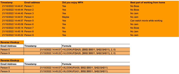
Dear all,
Check this out, it has been difficult to perform a reversed vlookup in both sheets and excel, now it's made easy by xlookup without any needs of manually reversing the columns in the range
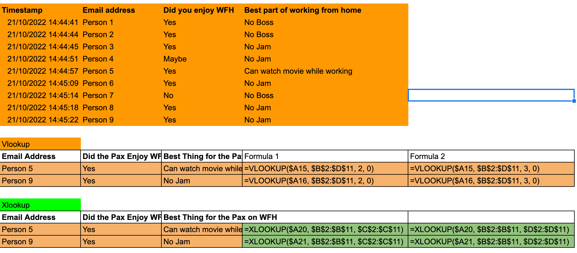
Dear All,
Xlookup has just been launched in Google sheets, this vlookup replacement function its much more simpler, bi-direction and easy to use.
Sample as below: